Map Projections, spatialreference.org and gdalwarp

Map Projections

The question of map projections and how to reproject data is one that comes up often in discussions with both experienced colleagues and those new to the geospatial profession. I’m not going to go through a complete discussion of map projections here, as there are many resources available on the Internet that can help you. I’m going to focus more on how to move data between projections.

At its most simple a map projection is simply a mathematical description of how to take data on the surface of a sphere, that are inherently 3-dimensional, and transform them to a 2-dimensional view. Here is a very early example of a map projection, courtesy of Claudius Ptolemy and Wikipedia.

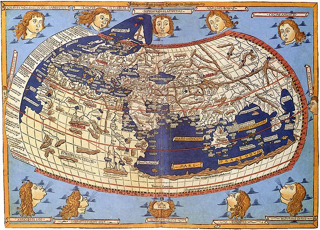
Of course, this isn’t a map projection in the sense we would define it now, but in its day it was as accurate as any. In Alaska, where I live, we use a variety of map projections for geospatial work. The most common of these are probably Universal Transverse Mercator (UTM), Albers Equal Area Alaska, Alaska State Plane, Northern Polar Stereographic, and of course the old standby WGS84 Lat/Lon. Each of these projections has it’s strengths and weaknesses and some are more appropriate for certain applications. If I’m working with land data in Alaska, I will often use UTM. The problem with UTM is that living at 65 degrees North latitude, the UTM zones change rapidly, as they are defined by the lines of longitude, which converge in the far North and South. Therefore, If I’m working with sea ice data in the Arctic Ocean, UTM will not work at all and I would probably use Northern Polar Stereographic, or perhaps WGS84 Lat/Lon.

SpatialReference

This is probably starting to get confusing and rightly so. There are hundreds, if not thousands, of projections ranging from being very specific for small areas to covering the entire globe. I live in UTM Zone 6N, and this is the OGC description of zone 6N.

PROJCS["WGS 84 / UTM zone 6N",
GEOGCS["WGS 84",
DATUM["WGS_1984",
SPHEROID["WGS 84",6378137,298.257223563,
AUTHORITY["EPSG","7030"]],
AUTHORITY["EPSG","6326"]],
PRIMEM["Greenwich",0,
AUTHORITY["EPSG","8901"]],
UNIT["degree",0.01745329251994328,
AUTHORITY["EPSG","9122"]],
AUTHORITY["EPSG","4326"]],
UNIT["metre",1,
AUTHORITY["EPSG","9001"]],
PROJECTION["Transverse_Mercator"],
PARAMETER["latitude_of_origin",0],
PARAMETER["central_meridian",-147],
PARAMETER["scale_factor",0.9996],
PARAMETER["false_easting",500000],
PARAMETER["false_northing",0],
AUTHORITY["EPSG","32606"],
AXIS["Easting",EAST],
AXIS["Northing",NORTH]]


That’s a lot to remember, and that brings us to the next part of this post, SpatialReference. Projection definitions can be very complex, but they don’t have to be hard to remember. You can either remember the information in the definition above, or you can remember the number 32606, which is the European Petroleum Survey Group (EPSG) code for UTM Zone 6N. In fact, the UTM northern zones are defined as 326XX, where XX is the zone number. So now, by remembering one zone, we have remembered all 60 of them. On spatialreference.org you can look up projections by name or by EPSG code.

How do we use this information? (i.e. gdalwarp)

My favorite tool for reprojecting data is gdalwarp. This is part of the GDAL suite, available at www.gdal.org. gdalwarp has many options that I can’t go into here. The most important for this discussion is -t_srs, which is the target projection definition. Luckily, we can simply define the output project by EPSG code as follows:

gdalwarp -s_srs EPSG:4326 -t_srs EPSG:32606 LatLonInputfile.tif UTM6NOutputFile.tif

In this example, the -s_srs is used to define the input projection and -t_srs defines the output projection. It’s really that simple. gdalwarp has many options that can be explored further HERE. The GDAL utility programs are some of my most often used tools and something every geospatial professional should have on their system.

As always, I hope you enjoyed this post and thank you for reading.

Some of my previous posts

Reading Geospatial Data with Python
QGIS Plugin – RasterCalc
QGIS Plugin – OpenLayers