GPX overview: An R function to create an overview of your .gpx files (using leaflet and RgoogleMaps)

Why GPX? For what?

It's convenient to record tracks of your hiking/field trips with the GPS of your smartphone, tablet or just GPS as .gpx files. You can use them to georeference your pictures (for example with the great georefencer of Digikam) or use them for any kind of mapping purpose. I'm mainly using Maverick (and sometimes the Offline Logger ) to do that, Maverick creates files named with the form "2015-08-26 @ 11-31-59.gpx", therefore I'm quickly collecting a large amount of such files.

Well, the name helps to find when the .gpx file was created but what if I want to find such a file made a long time ago? It's easy to open them one by one, with QGIS for example, and check what's inside, but if I don't remember the exact date of the file it can become a pain in the ass to find what I'm looking for.

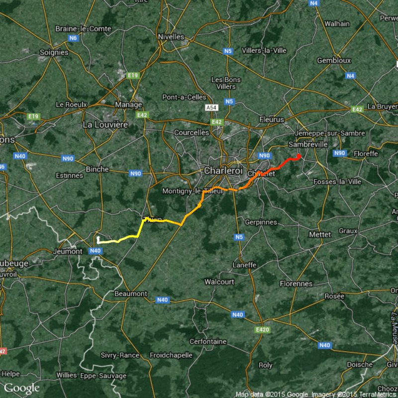
That's why I decided to write an R script creating a map with an overview of the recorded track, that I can run over a (long) list of files automatically. I started to write a short script using RgoogleMaps package producing, for each .gpx file, a map with the same name as the .gpx source. As a result, I get two folders, with the same number of files, one with all the .gpx and the second with all the .png maps, with corresponding names. Very convenient to browse through map overviews and find the GPS tracks I was seeking for.

However, in some case when a track includes very distant regions, the map is hard to read because of the large scale. This was the weakness of static maps and leaflet seemed to be the solution to easily make interactive maps that I can zoom/unzoom.
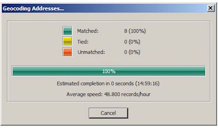
I adapted my script to include such a map into an .html file and I kept the static maps with different scales and backgrounds. As decorations for these maps, the script determines the first and last point's adresses and add it in the html, thanks to the reverse geocoding possibilities provided by the nice function reverseGeoCode() (J. Aswani, “All Things R: Geocode and reverse geocode your data using, R, JSON and Google Maps’ Geocoding API,” All Things R, 20-Mar-2012).
My function gives two kind of outputs: single .png map, a knitted .html page providing all details or both.
The way to decide which .gpx files to describe is rather flexible but partly associated with the way I organized the files on my comp. You may want to change this part for your own need.

And voilà for the context and the idea! It works like a charm, it takes a piece of time because I'm recalculating the speed of each (couple of) points... Well I know, speed is usually included inside of the .gpx attribute table, but I wanted to double check it. Just remove this part of the script if you want a faster process.

The .R code with the main function and the .Rmd code for knitting, are available on this GitHub repository. You're welcome to branch your improvements!

Let's describe how the function works.
Here we go!

File: 20150721_Apercu-GPX_Complet.R
Clean up and load libraries

rm(list=ls())
library(RgoogleMaps)
library(rgdal)
library(knitr)
library(leaflet)

Function 'reverseGeoCode()' of J. Aswani.

reverseGeoCode <- function(latlng) {
  latlngStr <-  gsub(' ','%20', paste(latlng, collapse=",")) #Collapse and Encode URL Parameters
  library("RJSONIO") #Load Library

Open Connection

  connectStr <- paste('http://maps.google.com/maps/api/geocode/json?sensor=false&amp;latlng=',latlngStr, sep="")
  con <- url(connectStr)
  data.json <- fromJSON(paste(readLines(con), collapse=""))
  close(con)

Flatten the received JSON

  data.json <- unlist(data.json)
  if(data.json["status"]=="OK")
    address <- data.json["results.formatted_address"]
  return (address)
}

The function 'GPX_Overview()':
* If "GPXname=NULL" the .gpx files processed are those which do not yet exist as .png (the names are collected in the vector 'AF').
Otherwize ,one or more .gpx file names can be provided as text vector.
* "option" should be specified whether to output only the .png map, to output the html report (with leaflet interactive map) or both.

GPX_Overview <- function(GPXname=NULL,option=c("SimplePNG","htmlReport","both")){

This part is specific to my own organization of the files (your folder where you store all your .gpx files)

  setwd("/home/jf/Dropbox/_Carto⁄LIFE-ELIA[dropBox]/Fichiers GPX/GPX2PNG") ### 

List of the .gpx files which were not yet processed

  GPXfile.list <- list.files()[grep(".gpx",list.files())]
  PNGfile.list <- list.files("./OutputPNG")[grep(".png",list.files("./OutputPNG"))]
  comp <- substring(PNGfile.list,1,25) ## Adapt substring start and stop to your .gpx name
  AF <- GPXfile.list[is.na(match(GPXfile.list,comp))]
  if(!is.null(GPXname)){AF <- GPXname} ## Choose .gpx files to process. This is the default, when no names are provided

sapply the script on each .gpx file. I had to use the '<<-' operator to keep some variables available when calling the .Rmd part for knitting. I suppose that other workarounds exist!?

  sapply(AF,function(GPXfile) {filename <<- GPXfile
  pts <<-  readOGR(GPXfile, layer = "track_points") # Read gpx file, layer 'track'

Keep the coordinates with 'native' CRS (WGS84) in decimal degrees

  crd.gpx <<- data.frame(pts@coords)
  colnames(crd.gpx) <<- c("Long", "Lat")

Reproject the coordinates into a metric system

  pts.crd <<- spTransform(pts,CRS("+init=epsg:3035"))@coords ### EUROPE

Produce map using RGoogleMaps library: I prepare two bounding boxes (bb and bb.w) to make two scales of maps.

  bb <<- qbbox(pts@bbox[2,],pts@bbox[1,], TYPE = "all",
               margin = list(m = rep(1, 4),TYPE = c("perc", "abs")[1]))
  range.lat <- 3*(bb$latR[2]-bb$latR[1])
  range.lon <- 3*(bb$lonR[2]-bb$lonR[1])
  bb.w <<- list(latR=c(bb$latR[1]-range.lat,bb$latR[2]+range.lat)
                ,lonR=c(bb$lonR[1]-range.lon,bb$lonR[2]+range.lon))

Create MyMap and export as .png background before plotting track points

  MyMap <<- GetMap.bbox(bb$lonR, bb$latR, destfile = paste(getwd(),"/OutputPNG/FondCarte/FondCarteGPX-",GPXfile,".png",sep="")
                        , maptype = "hybrid",size = c(640, 640))

Create subsets within among the dataset to draw the points with a gradient of colours (more readable on the map).

  Ncut <<- as.integer(sqrt(length(pts)))
  COL <<- cut(1:length(pts),Ncut,labels=heat.colors(Ncut))

Find the first identified address to get country name (used in naming the .png output)

  ads.beg <- NULL; nbeg <- 1
  while(!is.character(ads.beg)){ads.beg <- try(reverseGeoCode(crd.gpx[nbeg,2:1]))
  nbeg <- nbeg+1}
  SpltAds <- unlist(strsplit(ads.beg,", "))
  CNTRY <<- SpltAds[length(SpltAds)]

Simple .png output of the track on google hybrid background with PlotOnStaticMap()

  if(option=="SimplePNG" | option=="both"){
    png(paste(getwd(),"/OutputPNG/",GPXfile,"_",CNTRY, ".png",sep="")
        ,width=800,height=800)
    PlotOnStaticMap(MyMap, lat = crd.gpx$Lat, lon = crd.gpx$Long, size = c(640,640), cex = 1, pch = 20, col = as.character(COL), add = F)
    dev.off()}

Call .Rmd for knitting into .html

  if(option=="htmlReport" | option=="both"){
    MyMapWideHyb <<- GetMap.bbox(bb.w$lonR, bb.w$latR, destfile = paste(getwd(),"/OutputPNG/FondCarte/FondCarteGPX-",GPXfile,"Hyb_WIDE.png",sep=""), maptype = "hybrid",size = c(640, 640))
    MyMapWideTer <<- GetMap.bbox(bb.w$lonR, bb.w$latR, destfile = paste(getwd(),"/OutputPNG/FondCarte/FondCarteGPX-",GPXfile,"Ter_WIDE.png",sep=""), maptype = "terrain",size = c(640, 640))
    setwd('/home/jf/Dropbox (CARAH)/_Carto⁄LIFE-ELIA[dropBox]/Fichiers GPX/GPX2PNG/Output_html/')

Note!!: knit2html is not working with leaflet widget creation. The widget is not visible in the html page, only the message "!–html_preserve–".
=>; NOT RUN #knit2html(input='/home/jf/Dropbox (CARAH)/_Carto⁄LIFE-ELIA[dropBox]/Fichiers GPX/Apercu-GPX-Full_2html.Rmd',output=GPXfile,envir=globalenv())
The solution is explained on stack overflow:

    rmarkdown::render(input='/home/jf/R/GitHub/GPXView/Apercu-GPX-Full_2html.Rmd', output_dir='.',output_file=paste(GPXfile,'_',CNTRY,'.html',sep=""),envir=globalenv())
    setwd("/home/jf/Dropbox/_Carto⁄LIFE-ELIA[dropBox]/Fichiers GPX/GPX2PNG")
  }
  })
}

The Markdown

'Apercu-GPX-Full_2html.Rmd' is the markdown defining the .html content.

GPX file overview
-------------------------------------------
```{r 'Find Addresses',echo=FALSE}```
Nitems

First address identified:

ads.beg

Last address identified:

ads.end

Loop for computing the speed between two points. Skip this part if you need a faster process!
The delay between a point and the next one are computed in 'res'.
Euclidian distance between a point and the next one are computed in 'eucl'.

res

Speed in km/h

VIT

Get rid of artifacts of high speed ( > 250 km/h) due to bad sattelite coverage

VIT[VIT>250]

Define colors

Ncut

The next line, sourcing an additonal R script, is a trick to keep my MapBox token and MapID for myself 😉

source("/home/jf/Dropbox (CARAH)/_Carto⁄LIFE-ELIA[dropBox]/Fichiers GPX/MyMapID_and_Token.R")
leaflet() %>% addTiles(MyMapID_and_Token,group="MyMapbox") %>% addTiles(group="OSM") %>% addProviderTiles("OpenMapSurfer.Roads", group = "OpenMapSurfer.Roads") %>% addCircles(crd.gpx[,1],crd.gpx[,2], radius = 5,opacity=0.8,col='red') %>% addMarkers(lat=crd.POP$Lat,lng=crd.POP$Long,popup=POP,options=markerOptions(clickable=TRUE)) %>% addLayersControl(baseGroups = c("MyMapBox","OSM","OpenMapSurfer.Roads"))
```
Static maps with RgoogleMaps
-------------------------------

**Orthophoto background**

```{r 'Plot map orthophoto',echo=FALSE}
PlotOnStaticMap(MyMap, lat = crd.gpx$Lat, lon = crd.gpx$Long, size = c(640,640),
 cex = 1, pch = 20, col = as.character(COL.VIT), add = F)
```

**Terrain background (wide frame)** 
```{r 'Plot map terrain',echo=FALSE}
PlotOnStaticMap(MyMapWideTer, lat = crd.gpx$Lat, lon = crd.gpx$Long, size = c(640,640),
 cex = 1, pch = 20, col = as.character(COL.VIT), add = F)
```

**Google hybrid background (wide frame)**
```{r 'Plot map hybrid',echo=FALSE,eval=T}
PlotOnStaticMap(MyMapWideHyb, lat = crd.gpx$Lat, lon = crd.gpx$Long, size = c(640,640),
 cex = 1, pch = 20, col = as.character(COL.VIT), add = F)
```

Details of speed
-----------------------

```{r 'Draw histrogram and plot',echo=FALSE}
cpar

Results (examples provided on GitHub repository):

1. Simple map overview

1. Output as .html including the leaflet interactive map, static maps, graphs and stats about the speed.

These two (actually 3) scripts can definitely be much simpler. Here I wanted to have fun with the possibilities of RgoogleMaps and leaflet packages.
Unfortunately the leaflet interactive map is rather heavy for my comp when the tracks are made of more than 1000 points. But my comp is an old stuff!

### How to use the function GPX_Overview()
GPX_Overview(option="both") # Full output of all .gpx files that do not yet exist as .png maps.
GPX_Overview(option="htmlReport") # idem to output only the .html page.
GPX_Overview(GPXname="2014-06-05 @ 10-36-14.gpx",option="htmlReport") ## .html page only for one file

Files2View GPX_Overview(GPXname=Files2View,option="both")