
When I first thought about it and trying to get tweets from the Twitter API I reached any limits quite soon. So how was it possible to get over 10GB of twitter data in just 8hrs?
Collecting Twitter Data
After google showed me some workarounds that were not working I found this post and applied the logic to my situation:
import tweepy
import json
import jsonpickle
#get the following by creating an app on dev.twitter.com
consumer_key = 'your consumer key here'
consumer_secret = 'your consumer secret here'
auth = tweepy.AppAuthHandler(consumer_key, consumer_secret)
api = tweepy.API(auth, wait_on_rate_limit=True,wait_on_rate_limit_notify=True)
searchQuery = '#Turkey'  # this is what we're searching for
maxTweets = 100 # Some arbitrary large number
tweetsPerQry = 100  # this is the max the API permits
fName = '/tmp/tweetsgeo.txt' # We'll store the tweets in a text file.
sinceId = None
max_id = -1
print("Downloading max {0} tweets".format(maxTweets))
with open(fName, 'w') as f:
    while tweetCount < maxTweets:
        try:
            if (max_id <= 0):
                if (not sinceId):
                    new_tweets = api.search(q=searchQuery, count=tweetsPerQry, since=2016-07-15)
                else:
                    new_tweets = api.search(q=searchQuery, count=tweetsPerQry,
                                            since_id=sinceId, since=2016-07-15)
            else:
                if (not sinceId):
                    new_tweets = api.search(q=searchQuery, count=tweetsPerQry,
                                            max_id=str(max_id - 1), since=2016-07-15)
                else:
                    new_tweets = api.search(q=searchQuery, count=tweetsPerQry,
                                            max_id=str(max_id - 1),
                                            since_id=sinceId, since=2016-07-15)
            if not new_tweets:
                print("No more tweets found")
                break
            for tweet in new_tweets:
                f.write(jsonpickle.encode(tweet._json, unpicklable=False) +
                        '\n')
            tweetCount += len(new_tweets)
            print("Downloaded {0} tweets".format(tweetCount))
            max_id = new_tweets[-1].id
        except tweepy.TweepError as e:
            # Just exit if any error
            print("some error : " + str(e))
            break

print ("Downloaded {0} tweets, Saved to {1}".format(tweetCount, fName))
In the end I needed to set the maximum number of tweets very high… So I ended up with approx. 1’729’000 tweets and this made up a file of at least 10GB (CAUTION! zipped 1.2GB).
Tweets Origin
There are several ways to get a spatial information of a tweet. The most accurate might be the tweet location if someone uses the localization of his device (mostly on mobile I assume). The number of tweets is quite small (0.1% are with lat/lon) But nevertheless: Let me put them on a map:
Tweets Place
Sometimes the tweet does not have a real geocoordinate but the user “tagged” a place. We can also analyze this one:
#the data for places is less reliable but also good
data = []
import json
import pandas as pd
index = 0
with open('/your/place/merge.txt') as f:
for line in f:
index+=1
jsonline=json.loads(line)
if jsonline['place'] != None:
data.append([jsonline['place']['country']])
if index%50000==0:
print index
tweets = pd.DataFrame(data)
tweets.columns=(['country'])
tweets=pd.DataFrame({'tweets':tweets['country'].value_counts()})
tweet.to_json("/your/place/countries_grouped.json", orient='records')
As we can see in the map also most Tweets were tagged inside the US (4030), yet the most tweets per 1 Million citizens originated from Gibraltar (7), Qatar (144) and Maldives(44). Especially the high number of tweets from Qatar comes with a flavor thinking about the current interaction of the country into international terrorism.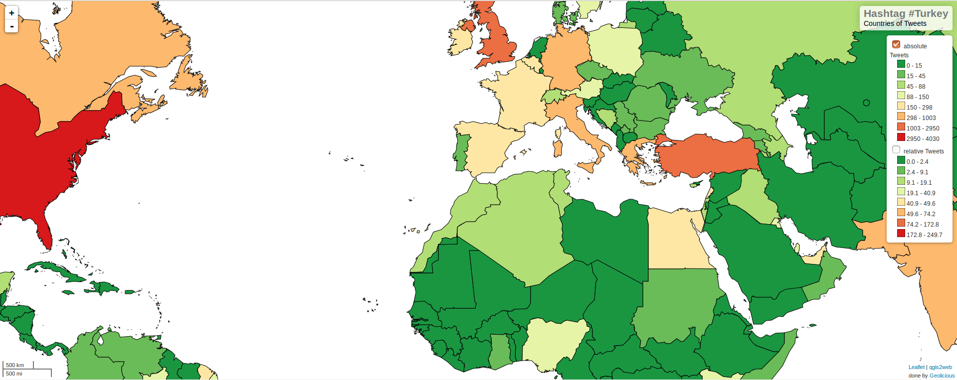
Time
As we already saw on the map the number of tweets increased significantly during the first news. News channels still not changed their program but #Turkey was definitely trending at that time: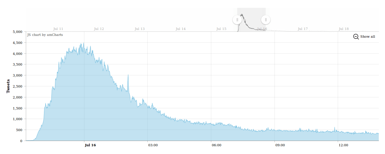
The code for getting and rounding the tweeting times:
from dateutil.parser import parse
import json
creation_times=[]
#for text analysis just store text and user:
data = []
with open('/your/place/merge.txt') as f:
    for line in f:
        jsonline=json.loads(line)
        data.append([jsonline['user']['name'],jsonline['text'],jsonline['created_at']])
        if len(data)%50000==0:
            print len(data)
for tweet in data:
    creation_times.append(parse(tweet[2]))
    if len(creation_times)%50000==0:
        print len(creation_times)
import datetime
import pandas as pd
rounded_times=[]
for time in creation_times:
    tm = time
    rounded_times.append(tm - datetime.timedelta(minutes=tm.minute % 1, seconds=tm.second, microseconds=tm.microsecond))
times=pd.DataFrame({'time':rounded_times})
times2=pd.DataFrame({'tweets':times['time'].value_counts()})
times2['time'] = times2.index
times2.sort_values('time').to_json("/your/place/times.json", orient='records')
further readingThe Conditioned Impact of Recession News: A Time‐Series Analysis of Economic Communication in the United States, 1987–1996,
Tweets Language
Most tweets are associated with English. This is set by the user and in the current tweet selection. Our results show a massive occurrence of English tweets: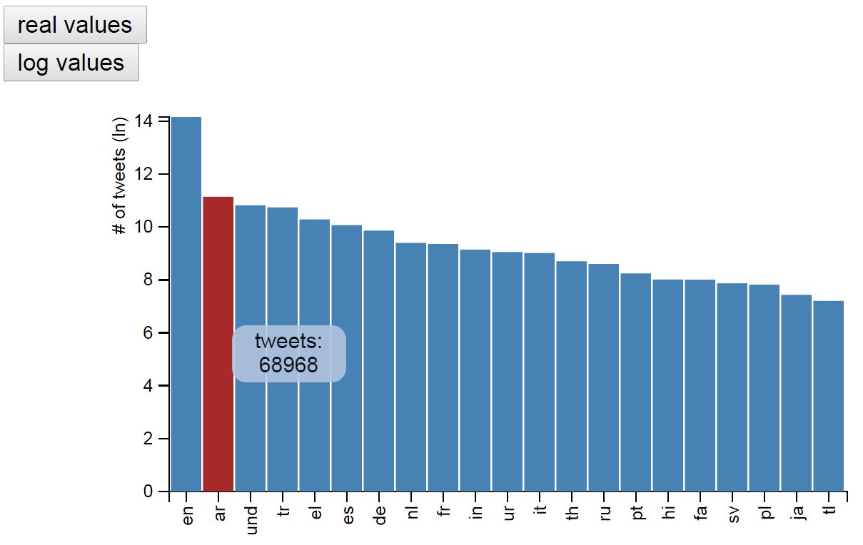
Tweet Text Analysis
The TTA I will do will cover an examination of retweets and “via” tweets in comparison to “original” tweets and a short term frequency analysis. According to this short code the number of individual tweets seems quite high with 338583 individual non retweeted tweets. I will examine this original content, remove stop words and count the 50 most frequent ones.
#assuming we have a file with tweets:
data = []
with open('/path/to/file.txt') as f:
    for line in f:
        jsonline=json.loads(line)
        data.append([jsonline['user']['name'],jsonline['text'],jsonline['created_at']])
        if len(data)%50000==0:
            print len(data)
text = []
for tweet in data:
    if "RT @" not in tweet[1]:
        text.append(tweet[1])
individual=' '.join(text)
from nltk.corpus import stopwords
import string
import nltk
punctuation = list(string.punctuation)
#nltk.download() #for first run needed
stop = stopwords.words('english') + punctuation + ['rt', 'via', 'the', 'turkey', 'coup','turkeyCoup']
non_stop_text = ' '.join([word.lower() for word in individual.split() if word.lower() not in stop and not word.startswith(('#', '@'))])
from collections import Counter
import pandas as pd
#count_all = Counter()
count_all=Counter(non_stop_text.split())
#count_all.update(non_stop_text.split())
toplist=count_all.most_common(50)
toplistpd = pd.DataFrame(toplist)
toplistpd.columns = ["word","count"]
toplistpd.to_json("/your/place/topwords.json", orient='records')
#non_stop_text[0:1000]
The word count is quite limited in its possibility of interpretation. Yet we need to state that the term democracy is under the top 20 and the “de” flag is more often used than the “en” flag assuming a connection between the EU deal with Turkey and the role of chancellor Merkel in the whole discussion and the rumor of RT Erdogan fleeing to Germany.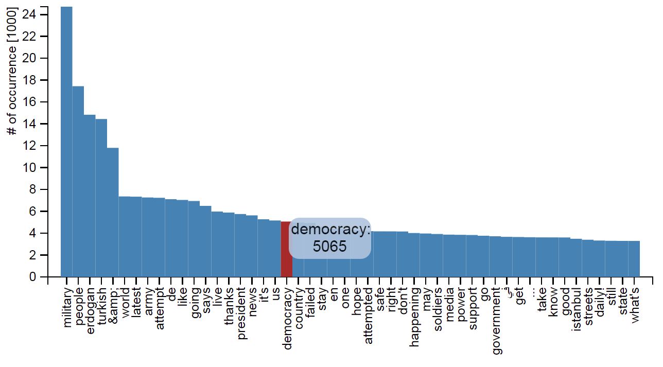

This is a great analysis!
Reminds me of the analysis that Floating Sheep did a few years back-
http://users.humboldt.edu/mstephens/hate/hate_map.html
Thanks for sharing out your code also,
Best,
Stephen
Very interesting, eventhough I always a bit sceptical about the validity of Twitter data since it is still a very selective group of people using it.
But still, have you thought about visualising word usage over time or per country? It might be interesting so see how the topic changed over time or people were concered over different topics.