Run GIS functions directly in Python with GeoPandas

GeoPandas, once installed, supports you with a handfull of GIS functions in your Python notebooks and will leverage your work with geospatial data. But to be honest: this wouldn’t be worth a notice. But the combination of GIS functions with other Pandas functions makes this module the new swiss army knife for geospatial work in scripts.

In this article I’ll show you the installation, present basic functions and provide you a notebook (written by Jakob) with the most basic operations for a nice “get-to-know”.

GeoPandas – Installation

You can add the GeoPandas modul in different ways to your Python environment. For this article I am using the pip way. If you prefer the Anaconda installation, you might follow this link or even try to install it from source. You’ll find plenty of ways on the GeoPandas webpage.

As I am working on a mac, I installed geos first using brew and used pip to install the GeoPandas extension for Pandas and to meet dependies. If you need the Jupyter notebook as well to follow, install it via pip as well:

brew install geos
brew install spatialindex
pip install jupyterlab
pip install geopandas
pip install rtree
pip install matplotlib

Now fire up a new Jupyter Notebook from the shell:

jupyter notebook

First steps with GeoPandas

Once you created a new notebook, we simply add the module together with Pandas:

import pandas as pd
import geopandas as gp

now, all the GeoPandas functions can be used in your notebook and we will try some of them with the country-dataset from naturalearthdata.com and all office locations of the world from osmdata.xyz (big props to Dr. Marz!). The command is damn easy:

# basic usage: gp.read_file(PATH_TO_YOUR_SHAPE_FILE(s))
countries = gp.read_file("ne_10m_admin_0_countries.shp") #as I've donwloaded it to the place where I started my notebook. 
offices = gp.read_file("office_EPSG4326.gpkg")

Working with the Attribute Table

Once the variables are defined and the files are read, the head function of this “geoDataFrame” will show you the first entries of a large dataset which keeps your notebook quite tidy compared to printing the whole attribute table:

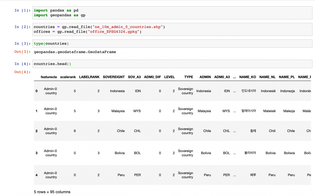
The head function returns 5 rows by default but you can also alter the number of by simply adding the number of rows:

offices.head(2)

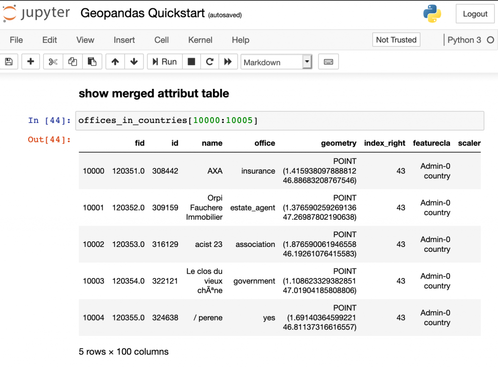
Now we’ll join both data sets.

Joining data in GeoPandas

Both variables share an spatial information and we use the spatial join (sjoin) to join the office feature set with the country dataset:

import rtree
officeCountries = gp.sjoin(offices, countries)

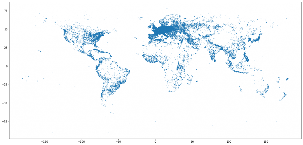
But as we love maps, let’s create a simple one:

import matplotlib
officeCountries.plot(markersize=0.05, figsize=(20,10))

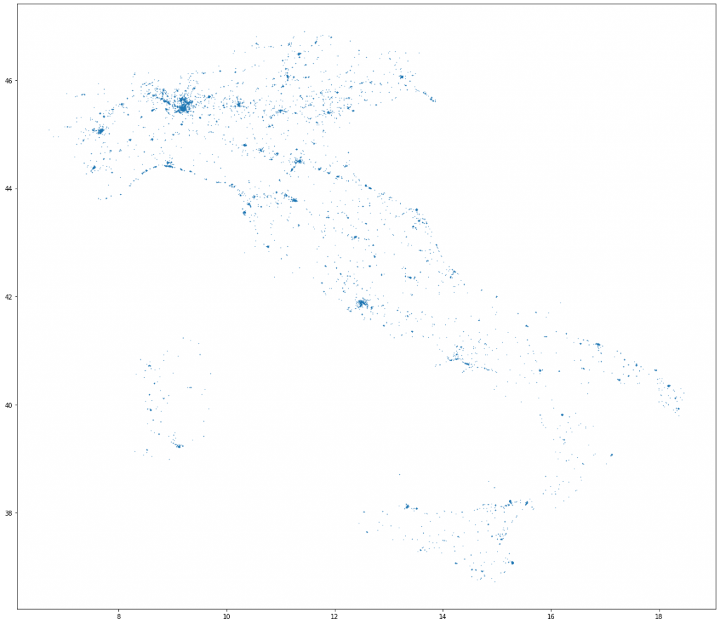
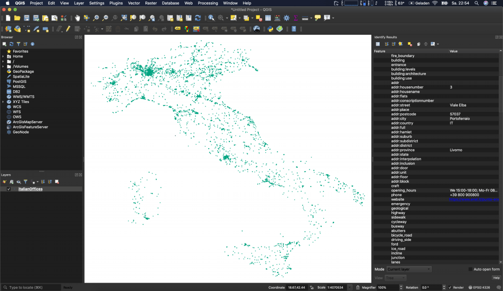
officeCountries[officeCountries.SOVEREIGNT == 'Italy'].plot(markersize=0.1, figsize=(20,20)) #italy only

Storing the Result

Now we created a new dataset as we merged country-attributes with office-attributes. So let’s store the information in a new file:

officeCountries[officeCountries.SOVEREIGNT == 'Italy'].to_file(driver = 'GeoJSON', filename= "italianOffices.geojson")

Doesn’t it look beautiful in QGIS?

To me GeoPandas comes in handy if I want to concentrate on data and not on cartograhic styling. So if you need to scrape some data, enrich it with spatial information or only want to read the attribute table of a good old shapefile without opening a full blown solution like QGIS or ESRI, GeoPandas comes in handy. Especially for some automatic workflows this is a great extension!

Enjoy your first steps with GeoPandas!